Model Interpreter via Contextual AI

In this tutorial, we use xai to analyze a trained model and its features. The tutorial contains 3 parts: - feature distribution analysis - trained model feature importance analysis - model interpretation via explanation aggregation

Prerequisites : Import libraries

xai.model.interpreter is the main package that users of Contextual AI interact with.

# Some auxiliary imports for the tutorial
import sys
import random
import numpy as np

from pprint import pprint
from sklearn import datasets
from sklearn.model_selection import train_test_split
from sklearn.ensemble import RandomForestClassifier

# Set seed for reproducibility
np.random.seed(123456)

# Set the path so that we can import ExplainerFactory
sys.path.append('../../')

# Main Contextual AI imports
import xai
from xai.model.interpreter.model_interpreter import ModelInterpreter

In this tutorial, we train a sample RandomForestClassifier model on the Wisconsin breast cancer dataset, a sample binary classification problem that is provided by scikit-learn (details can be found here). We will use APIs in xai.model_interpreter package to conduct feature analysis, feature ranking and model interpretation.

# Load the dataset and prepare training and test sets
raw_data = datasets.load_breast_cancer()
X, y = raw_data['data'], raw_data['target']
X_train, X_test, y_train, y_test = train_test_split(X, y, test_size=0.2)

1. Feature Analysis

Key parameters used in feature analysis: - feature_names: a list of str, names of each feature. - feature_types: a list of str, pre-defined type for each feature. - train_x: numpy.dnarray, training data. Each row is a training sample, each column is a feature. - labels: a list of str/int, the class label for each training sample. - trained_model: model object, the trained model object.

Feature Distribution

To analyze the feature distribution, we need to import xai.model_interpreter.FeatureInterpreter to initialize a FeatureInterpreter and call the get_feature_distribution() function.

# Define the feature data type and feature names
from xai.data.constants import DATATYPE
feature_names = raw_data['feature_names'].tolist()
feature_types = [DATATYPE.NUMBER]*len(feature_names)

from xai.model.interpreter.feature_interpreter import FeatureInterpreter
feature_interpreter = FeatureInterpreter(feature_names=feature_names)

stats = feature_interpreter.get_feature_distribution(feature_types=feature_types,train_x=X_train,labels=y_train)

We use our plot helper class NotebookPlots to plot the feature distribution results for the first 3 features. Details for each type of stats can be found in xai.data.explorer under different data type packages.

from xai.plots.data_stats_notebook_plots import NotebookPlots
plotter = NotebookPlots()

sample_features = feature_names[:3]
for feature_name in sample_features:
    (label_feature_stats, all_feature_stats) = stats[feature_name]

    plotter.plot_labelled_numerical_stats(labelled_stats=label_feature_stats, # stats for each class
                                          all_stats=all_feature_stats, # stats for all classes
                                          label_column='Class', # column name for label
                                          feature_column=feature_name) # column name for feature

mean radius

	class	min	max	mean	median	sd	total_count
0	1	6.981	16.84	12.095455	1.700759	16.84	286
1	0	11.420	28.11	17.468462	3.158721	28.11	169
2	all	6.981	28.11	14.091143	3.502028	28.11	455

mean texture

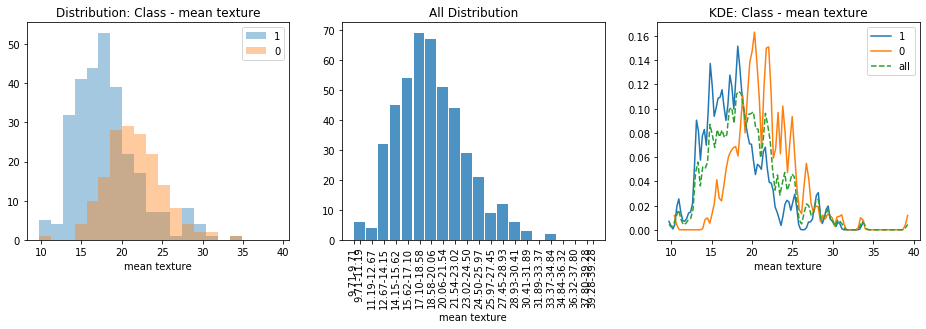
	class	min	max	mean	median	sd	total_count
0	1	9.71	33.81	18.066643	4.013245	33.81	286
1	0	10.38	39.28	21.600118	3.738992	39.28	169
2	all	9.71	39.28	19.379077	4.269827	39.28	455

mean perimeter

	class	min	max	mean	median	sd	total_count
0	1	43.79	108.4	77.730105	11.292902	108.4	286
1	0	75.00	188.5	115.335503	21.653977	188.5	169
2	all	43.79	188.5	91.697824	24.176163	188.5	455

Feature correlation

To analyze the feature correlction, we need to import xai.model_interpreter.FeatureInterpreter to initialize a FeatureInterpreter and call the get_feature_correlation() function. Same FeatureInterpreter object can be reused here for correlation analysis.

In this sample, as all the features are numerical features, correlation are calculated using Pearson’s testing as a default setup. And we use plot helper function to plot the heatmap for the correlation between all features.

types, values = feature_interpreter.get_feature_correlation(feature_types=feature_types,train_x=X_train)
plotter.plot_correlation_heatmap(types,values)

../../xai/model/interpreter/feature_interpreter.py:138: SettingWithCopyWarning:
A value is trying to be set on a copy of a slice from a DataFrame

See the caveats in the documentation: http://pandas.pydata.org/pandas-docs/stable/user_guide/indexing.html#returning-a-view-versus-a-copy
  correlation_types[col1][col2] = method
/Users/i309943/opt/anaconda3/envs/xai/lib/python3.6/site-packages/pandas/core/indexing.py:202: SettingWithCopyWarning:
A value is trying to be set on a copy of a slice from a DataFrame

See the caveats in the documentation: http://pandas.pydata.org/pandas-docs/stable/user_guide/indexing.html#returning-a-view-versus-a-copy
  self._setitem_with_indexer(indexer, value)

Correlation Type: pearson

2. Feature Importance

As feature importance is associated with a model, we need to firstly train a sample model first. In this tutorial, we train a sample RandomForestClassifier model on the the dataset.

# Instantiate a classifier, train, and evaluate on test set
clf = RandomForestClassifier()
clf.fit(X_train, y_train)
clf.score(X_test, y_test)

/Users/i309943/opt/anaconda3/envs/xai/lib/python3.6/site-packages/sklearn/ensemble/forest.py:245: FutureWarning: The default value of n_estimators will change from 10 in version 0.20 to 100 in 0.22.
  "10 in version 0.20 to 100 in 0.22.", FutureWarning)

0.956140350877193

To analysze the feature importance ranking, we need to import xai.model_interpreter.FeatureInterpreter to initialize a FeatureInterpreter and call the get_feature_ranking() function. Same FeatureInterpreter object can be reused here for feature importance ranking.

The code below shows the feature importance used the default method provided by the model itself.

feature_importance_ranking = feature_interpreter.get_feature_importance_ranking(trained_model=clf,
                                                                                train_x=X_train,
                                                                                method='default')
plotter.plot_feature_importance_ranking(feature_importance_ranking)

By changing the method, we can get feature importance based on different criterion. The code below shows the feature importance calculated by shap value.

feature_importance_ranking = feature_interpreter.get_feature_importance_ranking(trained_model=clf,
                                                                                train_x=X_train,
                                                                                method='shap')
plotter.plot_feature_importance_ranking(feature_importance_ranking)

We can also plot the shap values in a summary plot to show individual sample shap values for all the features.

feature_shap_values = feature_interpreter.get_feature_shap_values(trained_model=clf,
                                                                  train_x=X_train)

plotter.plot_feature_shap_values(feature_shap_values,class_id = 1, X_train=X_train)

3. Model Interpretation by aggregate explanations

One way to interpret the model is by aggregating the individual explanations which tries to explain the model locally

Step 0. Import the ModelInterpreter

from xai.model.interpreter.model_interpreter import ModelInterpreter

Step 1. Define domain and algorithm

As model interpreter is using a model-agnostic explainer, domain and algorithm is dependent on xai.explainer package. See details in xai.explainer.config

from xai.explainer.config import DOMAIN, ALG
model_interpreter = ModelInterpreter(domain=DOMAIN.TABULAR, algorithm=ALG.LIME)

Step 2. Build interpreter

Based on the domain and algorithm chosen, build the explainer in the interpreter by passing in the required parameter.

Required parameters include: - training data - training labels - model prediction functions

See details in xai.explainer.

model_interpreter.build_interpreter(
    training_data=X_train,
    training_labels=y_train,
    mode=xai.MODE.CLASSIFICATION,
    predict_fn=clf.predict_proba,
    feature_names=raw_data['feature_names'],
    class_names=list(raw_data['target_names'])
)

Step 3. Interpreter the model with training data

Model Interpretation

The interpreter explains the model by aggregate explainations based on predicted classes. By calling interpret_model() with training data, the explainer will explain each sample on a local manner and aggregate the local explanations on each class to provide a global interpretation statistically. For now, we support 3 types of statistical aggregation: - top_k: how often a feature appears in the top K features in the explanation - average_score: average score for each feature in the explanation - average_ranking: average ranking for each feature in the explanation

Default type is top_k.

stats = model_interpreter.interpret_model(samples=X_train, stats_type='top_k',k=5)

../../xai/model/interpreter/model_interpreter.py:83: UserWarning: Interpret 100/455 samples
  idx + 1, len(samples)))
../../xai/model/interpreter/model_interpreter.py:83: UserWarning: Interpret 200/455 samples
  idx + 1, len(samples)))
../../xai/model/interpreter/model_interpreter.py:83: UserWarning: Interpret 300/455 samples
  idx + 1, len(samples)))
../../xai/model/interpreter/model_interpreter.py:83: UserWarning: Interpret 400/455 samples
  idx + 1, len(samples)))

class_stats, total_count = stats
num_of_top_explanation = 15
for _class,_explanation_ranking in class_stats.items():
    print('Interpretation for Class %s'%_class)
    plotter.plot_feature_importance_ranking([(key,value) for key,value in _explanation_ranking.items()]
                                            [:num_of_top_explanation])

Interpretation for Class 1

Interpretation for Class 0

Error Analaysis

Error analysis helps to aggregate explanations on samples that are wrongly classified in the validation data set.

By calling function error_analysis(), it returns a stats of top explanations for wrongly classified samples.

stats = model_interpreter.error_analysis(class_num=2, valid_x=X_test, valid_y=y_test, stats_type='average_score', k=5)

../../xai/model/interpreter/model_interpreter.py:128: UserWarning: Analyze 10/114 samples
  idx + 1, len(valid_x)))
../../xai/model/interpreter/model_interpreter.py:128: UserWarning: Analyze 20/114 samples
  idx + 1, len(valid_x)))
../../xai/model/interpreter/model_interpreter.py:128: UserWarning: Analyze 30/114 samples
  idx + 1, len(valid_x)))
../../xai/model/interpreter/model_interpreter.py:128: UserWarning: Analyze 40/114 samples
  idx + 1, len(valid_x)))
../../xai/model/interpreter/model_interpreter.py:128: UserWarning: Analyze 50/114 samples
  idx + 1, len(valid_x)))
../../xai/model/interpreter/model_interpreter.py:128: UserWarning: Analyze 60/114 samples
  idx + 1, len(valid_x)))
../../xai/model/interpreter/model_interpreter.py:128: UserWarning: Analyze 70/114 samples
  idx + 1, len(valid_x)))
../../xai/model/interpreter/model_interpreter.py:128: UserWarning: Analyze 80/114 samples
  idx + 1, len(valid_x)))
../../xai/model/interpreter/model_interpreter.py:128: UserWarning: Analyze 90/114 samples
  idx + 1, len(valid_x)))
../../xai/model/interpreter/model_interpreter.py:128: UserWarning: Analyze 100/114 samples
  idx + 1, len(valid_x)))
../../xai/model/interpreter/model_interpreter.py:128: UserWarning: Analyze 110/114 samples
  idx + 1, len(valid_x)))

num_of_top_explanation = 10
for (gt_class,predict_class),(_explanation_dict,num_sample) in stats.items():
    print('%s sample from class [%s] is wrongly classified as class[%s]'%(num_sample,gt_class,predict_class))
    print(' - Top reasons that they are predicted as class[%s]'%predict_class)
    plotter.plot_feature_importance_ranking([(key,value) for key,value in _explanation_dict[predict_class].items()]
                                            [:num_of_top_explanation])

3 sample from class [1] is wrongly classified as class[0]
 - Top reasons that they are predicted as class[0]

2 sample from class [0] is wrongly classified as class[1]
 - Top reasons that they are predicted as class[1]